
Article by Mattia Favretto – Full-stack Developer at AzzurroDigitale
Let’s discover how it is possible to print solid objects while minimising material waste and increasing production efficiency thanks to advanced nesting software.
In the manufacturing world, space is money. Every square centimetre of wasted material or unused volume translates into a direct loss. This is where Nesting comes into play: not just a simple interlocking of shapes, but a complex mathematical challenge aimed at minimising waste.
There are different types of nesting. The most common is 2D Nesting, typical of sheet metal or fabric cutting, where flat shapes are arranged on a surface. At the opposite extreme is 3D Nesting, where the best positioning for solid shapes is sought, which is extremely complex computationally.
In between, however, there is a specific challenge that we have addressed: 2.5D Nesting. In this scenario, we start with three-dimensional objects (CAD files) that must be arranged on a plane, but whose arrangement is constrained not only by their footprint, but also by their heights and spatial geometric characteristics. The scientific literature is vast, but often theoretical; implementing an industrial solution requires overcoming the barrier between academic theory and production reality.
The adoption of an advanced nesting algorithm is not a technological fad, but a strategic lever for competitiveness.
- Quality standardisation: While human efficiency can vary depending on fatigue or experience, the algorithm guarantees a constant search for the optimal solution, ensuring predictable and repeatable results.
- Reduction of direct costs: The primary objective is to reduce raw material waste. By optimising the positioning of the pieces, more products can be placed on the same sheet or in the same load volume, drastically reducing waste material.
- Automation and speed: Processes that would require hours of manual attempts by experienced operators are resolved in a short time, freeing up human resources for tasks with greater added value.
How It Works: simplifying complexity
Imagine playing Tetris, but with much more difficult rules: the pieces are not simple geometric blocks, but irregular, curved and complex shapes.
Our solution tackles the problem in three logical steps:
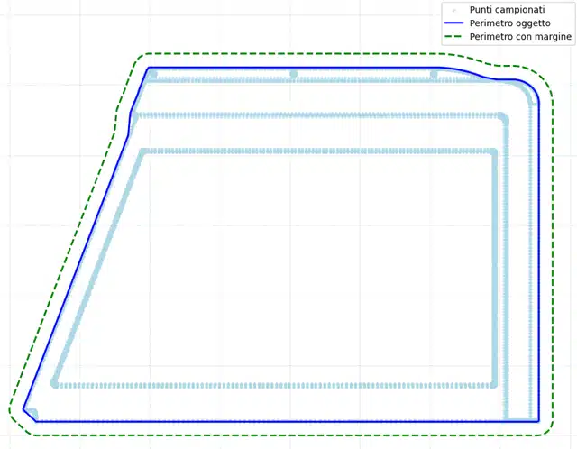
1. Collision prevention (safety margin): Before fitting the pieces together, the software adds a small buffer, a safety margin around the perimeter of each shape. This measure is not only necessary for production purposes but also compensates for small mathematical inaccuracies and prevents the pieces from accidentally touching or overlapping during positioning.
2. Recognition (from 3D to 2D): The system does not just see a flat outline. It analyses the original CAD file (STEP format) and extracts its footprint (the outer perimeter), also keeping track of heights. It is as if we were taking an X-ray of the object to understand how much space it actually occupies.
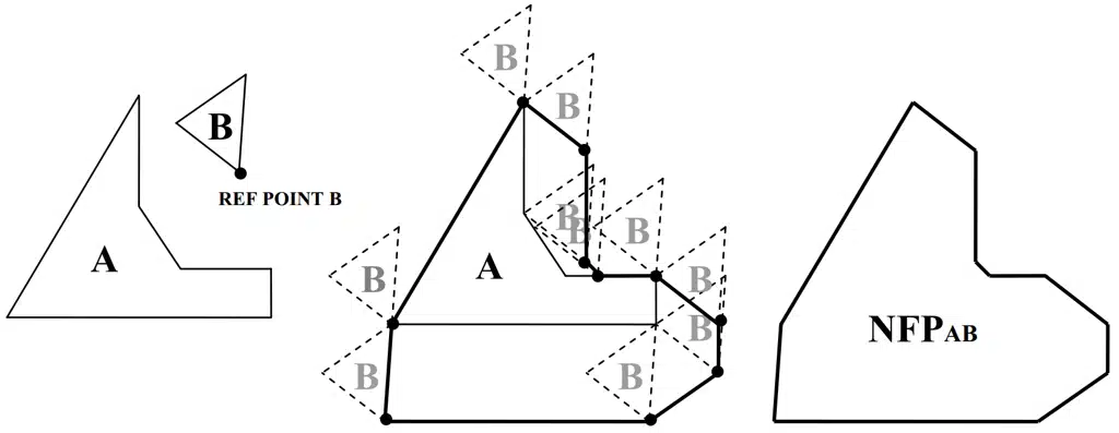
3. NFP geometry: To understand whether two pieces fit together, the software calculates a mathematical ‘prohibited’ area around each piece already placed (A). If the new piece (B) enters this area, it means there is a collision; if the new piece touches the edge of the area, we have perfect contact. The goal is to slide the new piece as close as possible to the existing ones without ever entering the forbidden zone.
4. The optimisation game: Once you understand how to fit two pieces together, you have to decide which piece to insert and where. The algorithm tries thousands of different combinations: it rotates the pieces, changes the order of insertion and “shakes” the solution when it realises it is stuck, all in order to find the configuration that takes up as little space as possible.
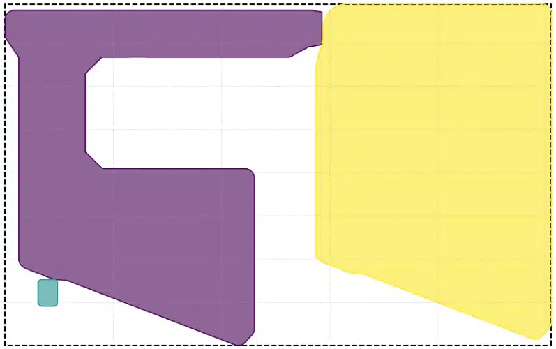
The objects shown here have a safety edge so that they do not touch each other even when they are close together
Deep Tech for Insiders
Our technical implementation is written in Python and uses advanced libraries for geometric manipulation and heuristic optimisation. Considering that nesting is a variant of the Bin Packing problem, classified as NP-Hard (therefore with non-polynomial complexity), in the search for the result it is necessary to resort to a sub-optimal solution since the search for the best solution would require excessive time, which is not applicable in our case.
1. CAD processing and 2.5D generation
The challenge begins with raw STEP files. We use the PythonOCC library to import the 3D geometry and analyse it.
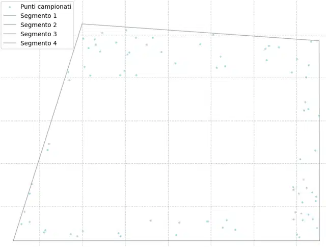
- Projection and Alpha Shape: The algorithm samples points along the edges of the faces of the 3D model and projects them onto the base plane. The perimeter of the figure is calculated on these points.
- Height mapping: We do not limit ourselves to the perimeter to understand how tall the object is. We identify the segments that best simplify our figure and calculate the height of each one, also taking into account the geometry of the polygon; this allows us to correctly evaluate the possible height variations present in a single piece. In particular, we construct a rectangular area for each side and randomly select points from which we calculate the height, then using a weighted upper average (it is better to err on the side of excess than deficiency), we associate a height with each side.
2. The geometric heart: No-Fit Polygon (NFP)
For positioning, we use the concept of No-Fit Polygon (NFP)1. Instead of continuously checking whether the new piece collides with those already in place, the software first generates a special template. This template, which is based on a geometric calculation called Minkowski Difference, represents the exact forbidden space around the fixed pieces. In practice, it is the footprint that the new piece would leave if it moved along the edges of those already placed, indicating the positions of perfect contact.
We use the Pyclipper library to perform these complex Boolean operations efficiently.
The resulting NFP zone represents the set of all positions where the centre of gravity of the moving part cannot go. Consequently, the contours of this zone represent the positions of perfect contact.
The algorithm selects the best candidates from the NFP geometry, favouring bottom-left positions to compact the layout towards the origin and reduce waste. The choice of valid positions for the pieces must take into account the height constraint. A search is then made for adjacent pieces and, if their heights differ excessively, a penalty is applied to the solution found, which is greater the greater the difference in height, thus allowing solutions whose heights slightly exceed the imposed limit not to be completely discarded.
3. GLS (Guided Local Search) optimisation algorithm
We do not rely on a simple greedy approach. We have implemented a Guided Local Search (GLS) meta-heuristic.
Local Mutations: The algorithm explores the solution space by applying mutations to the original sequence through rotations, exchanges of pieces and groups of pieces.
Constraint management: The algorithm applies higher costs to solutions that violate the set height constraints, making them less favourable but still possible if the waste is very low.
Restart and Perturbation: To avoid local minima, the system monitors improvements. If no better solution is found after a certain number of iterations, a massive permutation is triggered. This phase completely shuffles the sequence and assigns random rotations, forcing the algorithm to explore a completely new area of the solution space, temporarily accepting even worse solutions in order to break the deadlock.
Developer Glossary
- No-fit polygon (NFP): This is the prohibited area that forms around an already placed part (A), within which the reference point of a new part (B) cannot enter. Positioning the reference point of B:

To create the NFP in our algorithm, we use the centroid of the part, but this can be calculated with respect to each reference point of part B.
On the edge of the NFP: parts A and B are in perfect contact (interlocking).
Inside the NFP: parts A and B overlap (collision).
In order to minimise the area occupied by part B, I will choose a point on the edge of the NFP as its position. ↩︎
